人工智能实验报告
姓名: 徐国超
班级: 计算机2305
学号:
本报告分别从实验目的与内容、算法设计、核心代码实现、运行结果以及实验结论五个方面展示了两个实验的内容,并在报告最后附上了完整代码。
实验一:状态空间搜索算法编程实现(重排九宫问题)
实验目的与内容
实验中要求通过状态空间搜索算法编程实现一个具体问题,本报告选取经典的重排九宫问题,分别实现盲目搜索算法(BFS)与启发式搜索算法(A*)。并对两种算法在搜索节点数和耗时上的差异进行对比,理解启发式搜索在缩小搜索空间中的作用。
算法设计
- 有解性判断:本文程序在进行状态空间搜索之前,会首先计算序列的逆序对来判断该问题是否可解。若初始状态与目标状态逆序数奇偶性相同,则该状态可达,问题有解,反之则无解。
- 盲目搜索(BFS):使用先进先出队列存储待扩展节点,另外广度优先搜索可以保证在有解的情况下找到的解是最短路径。
- 启发式搜索(A)*:
- 启发函数:采用曼哈顿距离,计算每个数字当前位置与目标位置的行列距离之和。
- 评价函数:
,其中 为实际路径代价, 为启发函数,这里为曼哈顿距离。 - 数据结构:使用优先队列来对待扩展节点从小到大排序,确保每次扩展
最小的节点。
核心代码实现
def heuristic(self, state):
    distance = 0
    for i, val in enumerate(state):
        if val == 0: continue
        target_idx = val - 1
        curr_row, curr_col = i // 3, i % 3
        target_row, target_col = target_idx // 3, target_idx % 3
        distance += abs(curr_row - target_row) + abs(curr_col - target_col)
    return distance

def solve_astar(self):
    print("\nA*:")
    start_time = time.time()
    initial_h = self.heuristic(self.initial_state)
    pq = [(initial_h, 0, self.initial_state, [])]
    visited = {self.initial_state: 0}#记录到达该状态的最小g值

    nodes_explored = 0
    while pq:
        f, g, current_state, path = heapq.heappop(pq)
        nodes_explored += 1

        if current_state == GOAL_STATE:
            print(f"A*耗时: {time.time() - start_time:.4f}秒, 共搜索节点数: {nodes_explored}")
            return path

        for next_state, move in self.get_next(current_state):
            new_g = g + 1
            if next_state not in visited or new_g < visited[next_state]:
                visited[next_state] = new_g
                h = self.heuristic(next_state)
                heapq.heappush(pq, (new_g + h, new_g, next_state, path + [move]))
    return None
这段代码实现了基于曼哈顿距离的 A* 启发式搜索算法。其核心在于 heuristic 函数通过计算每个非零数字滑块当前位置与目标位置的行列坐标绝对差之和,为搜索提供了估计代价 solve_astar 执行过程中,算法利用优先队列动态维护评价函数 visited 字典实时记录并更新到达各状态的最小路径代价
运行结果
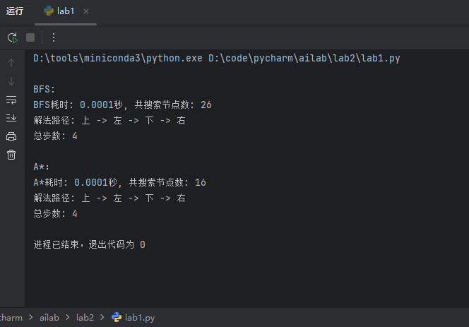
从图中可以看出,对于相同的重排九宫初始状态,广度优先搜索与 A* 算法均成功找到了步数为 4 的最短解路径。但在搜索效率的对比上,属于盲目搜索的广搜为了得到最优路径共搜索了 26 个节点,而属于启发式搜索的 A* 算法仅搜索了 16 个节点便找到了最优路径,节点搜索量减少了约 38.5%。这一结果直观地证明了启发式搜索在处理复杂状态空间问题时,能够通过收窄搜索范围、降低资源开销,展现出远高于盲目搜索的效率。
实验结论
通过对相同初始状态进行测试,结果表明:
- BFS 在有解的情况下可以保证找到最优解,但其搜索不带方向性,搜索的节点数量较大,消耗的资源大,效率相比来说更低。
- A* 算法通过曼哈顿距离的启发式引导,极大地减少了搜索范围,搜索效率更高。
实验二:神经网络分类器编程实现(BP算法)
实验目的与内容
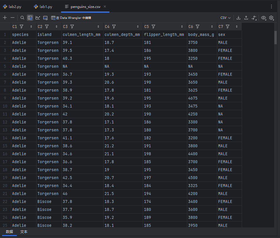
本实验要求手动编程实现人工神经网络中的反向传播算法,即构建一个 BP 神经网络,并解决一个实际分类问题。因此本报告在Kaggle上选取了一个数据集用于本次实验(https://www.kaggle.com/datasets/parulpandey/palmer-archipelago-antarctica-penguin-data)。该数据集是一份来自Palmer Archipelago (Antarctica)的企鹅数据,共有species、culmen_length_mm、culmen_depth_mm、flipper_length_mm、body_mass_g、island和sex共七个变量,本报告实现了通过其余六个变量该企鹅的species进行分类。
算法设计
- 网络架构:
- 输入层:7个特征(包括体征数据、性别、岛屿位置)。其中岛屿位置采用哑变量编码,本实验中的
island变量包含三个类别(Biscoe, Dream, Torgersen),在特征提取时,仅保留了其中两个(island_Biscoe和island_Dream)作为输入特征,这样可以讲岛屿类别的字符串类型转换成数字运算,并减少输入层维度,避免特征之间高度线性相关对模型收敛产生的不利影响。 - 隐藏层 1 (16 神经元) 和 隐藏层 2 (8 神经元):激活函数采用 ReLU,可以尽量预防出现梯度消失问题,并提高非线性拟合能力。
- 输出层 (3 神经元):对应3类企鹅,激活函数采用 Softmax,将输出转化为各预测类别的概率分布。
- 输入层:7个特征(包括体征数据、性别、岛屿位置)。其中岛屿位置采用哑变量编码,本实验中的
- 损失函数:采用交叉熵损失,其表达式为:$$L = -\frac{1}{m} \sum_{i=1}^{m} \sum_{j=1}^{C} y_{ij} \ln(\hat{y}_{ij})$$
相较于均方误差,交叉熵在输出层配合 Softmax 激活函数时,能够有效解决分类问题中的梯度弥散现象。并且在当预测值与真实值偏差较大时,交叉熵的梯度更明显,能显著加快BP算法的收敛速度。 - 数据处理:
- 缺失值处理: 代码采用df.ffill()前向填充策略。该方法利用数据序列中的前一个有效观测值来填充当前的空值,避免直接删除样本导致的信息减少。
- 类别特征编码:对目标变量species使用LabelEncoder。例如将文本类别的企鹅品种映射为整数数值(0, 1, 2),便于进行交叉熵计算。还对离散特征island进行处理,通过准则将其转换为二进制向量。
- 数值特征标准化:为了消除不同数据间的量纲影响,本报告采用StandardScaler对数据进行Z-score标准化,这防止了权重的梯度更新被大数值特征主导,使得梯度下降更加平稳。
核心代码实现
	def backward(self, X, y, output):
	    # 反向传播
	    m = y.shape[0]

	    # 输出层梯度
	    dz3 = output
	    dz3[range(m), y] -= 1
	    dz3 /= m

	    # 第二隐藏层梯度
	    dW3 = np.dot(self.a2.T, dz3)
	    db3 = np.sum(dz3, axis=0, keepdims=True)
	    da2 = np.dot(dz3, self.W3.T)

	    # ReLU梯度
	    da2[self.z2 <= 0] = 0

	    # 第一隐藏层梯度
	    dW2 = np.dot(self.a1.T, da2)
	    db2 = np.sum(da2, axis=0, keepdims=True)
	    da1 = np.dot(da2, self.W2.T)
	    da1[self.z1 <= 0] = 0

	    # 输入层梯度
	    dW1 = np.dot(X.T, da1)
	    db1 = np.sum(da1, axis=0, keepdims=True)

	    return dW1, db1, dW2, db2, dW3, db3

    def update_params(self, grads, learning_rate=0.01):
	    dW1, db1, dW2, db2, dW3, db3 = grads
	    self.W1 -= learning_rate * dW1
	    self.b1 -= learning_rate * db1
	    self.W2 -= learning_rate * dW2
	    self.b2 -= learning_rate * db2
	    self.W3 -= learning_rate * dW3
	    self.b3 -= learning_rate * db3

for epoch in range(epochs):
    output = nn.forward(X_train)
    loss = nn.compute_loss(output, y_train)
    grads = nn.backward(X_train, y_train, output)
    nn.update_params(grads, learning_rate=0.02)
这段核心代码主要展现了 BP 神经网络的核心学习机制:反向传播与参数优化。backward 函数基于链式法则,从输出层开始逐层向输入层计算损失函数对各个权重和偏置的梯度,其中包含了对 ReLU 激活函数梯度的处理;随后,update_params 函数利用计算出的梯度,通过梯度下降法按学习率更新网络参数。在主循环中,模型通过不断重复前向预测—计算损失—反向传播—更新权重的迭代过程,使得损失函数逐步减小,从而持续优化网络的分类性能。
运行结果
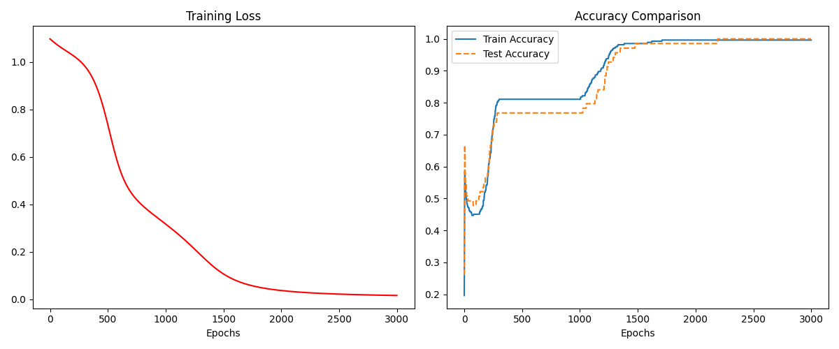
- 学习率:0.01;epochs:3000
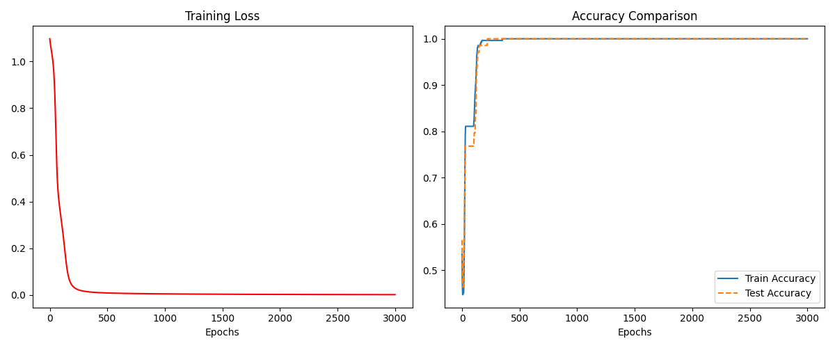
- 学习率:0.1;epochs:3000
实验结论
在学习率为 0.01 时,Loss 曲线下降较为平缓,准确率在大约 2200 个 Epoch 后趋于稳定;学习率提升至 0.1 时,模型在 500 个 Epoch 内便实现了损失函数近乎归零,且训练集与测试集的准确率均迅速达到 几乎100%,表明在合理范围内增大学习率能有效缩短训练时间,提高效率。同时,两组实验在测试集上的准确率曲线均能紧跟训练集,未出现明显的过拟合现象,证明了该 BP 神经网络分类器在当前数据集上具有极佳的泛化能力和鲁棒性。
完整代码
lab1:状态空间搜索算法编程实现
import heapq
from collections import deque
import time

GOAL_STATE = (1, 2, 3, 8, 0, 4, 7, 6, 5)
MOVES = {
    '左': (0, -1), '上': (-1, 0), '右': (0, 1),'下': (1, 0),
}


class Solve:
    def __init__(self, initial_state):
        self.initial_state = tuple(initial_state)

    def get_next(self, state):
        state_list = list(state)
        idx = state_list.index(0)
        row, col = idx // 3, idx % 3
        neighbors = []

        for move_name, (dr, dc) in MOVES.items():
            new_row, new_col = row + dr, col + dc
            if 0 <= new_row < 3 and 0 <= new_col < 3:
                new_idx = new_row * 3 + new_col
                new_state = list(state_list)
                new_state[idx], new_state[new_idx] = new_state[new_idx], new_state[idx]
                neighbors.append((tuple(new_state), move_name))
        return neighbors

    def print_path(self, path):
        print(f"解法路径: {' -> '.join(path)}")
        print(f"总步数: {len(path)}")

    def solve_bfs(self):
        print("\nBFS:")
        start_time = time.time()
        queue = deque([(self.initial_state, [])])
        visited = set([self.initial_state])

        explored = 0
        while queue:
            current_state, path = queue.popleft()
            explored += 1

            if current_state == GOAL_STATE:
                print(f"BFS耗时: {time.time() - start_time:.4f}秒, 共搜索节点数: {explored}")
                return path

            for next_state, move in self.get_next(current_state):
                if next_state not in visited:
                    visited.add(next_state)
                    queue.append((next_state, path + [move]))
        return None

    def heuristic(self, state):
        distance = 0
        for i, val in enumerate(state):
            if val == 0: continue
            target_idx = val - 1
            curr_row, curr_col = i // 3, i % 3
            target_row, target_col = target_idx // 3, target_idx % 3
            distance += abs(curr_row - target_row) + abs(curr_col - target_col)
        return distance

    def solve_astar(self):
        print("\nA*:")
        start_time = time.time()
        initial_h = self.heuristic(self.initial_state)
        pq = [(initial_h, 0, self.initial_state, [])]
        visited = {self.initial_state: 0}  # 记录到达该状态的最小g值

        nodes_explored = 0
        while pq:
            f, g, current_state, path = heapq.heappop(pq)
            nodes_explored += 1

            if current_state == GOAL_STATE:
                print(f"A*耗时: {time.time() - start_time:.4f}秒, 共搜索节点数: {nodes_explored}")
                return path

            for next_state, move in self.get_next(current_state):
                new_g = g + 1
                if next_state not in visited or new_g < visited[next_state]:
                    visited[next_state] = new_g
                    h = self.heuristic(next_state)
                    heapq.heappush(pq, (new_g + h, new_g, next_state, path + [move]))
        return None

    def is_solvable(self):
        def get_inversions(state):
            flat = [x for x in state if x != 0]
            count = 0
            for i in range(len(flat)):
                for j in range(i + 1, len(flat)):
                    if flat[i] > flat[j]:
                        count += 1
            return count % 2

        return get_inversions(self.initial_state) == get_inversions(GOAL_STATE)

if __name__ == "__main__":
    #初始状态
    #2 8 3
    #1 0 4    #7 6 5    start = (2, 8, 3, 1, 0, 4, 7, 6, 5)
    solver = Solve(start)

    # 检测是否有解
    if not solver.is_solvable():
        print("该初始状态无解")
    else:
        bfs_path = solver.solve_bfs()
        if bfs_path: solver.print_path(bfs_path)

        astar_path = solver.solve_astar()
        if astar_path: solver.print_path(astar_path)
lab2:神经网络分类器编程实现
import numpy as np
import pandas as pd
import matplotlib.pyplot as plt
from sklearn.model_selection import train_test_split
from sklearn.preprocessing import StandardScaler, LabelEncoder


class BP:
    def __init__(self, input_size, hidden1_size, hidden2_size, output_size):
        #初始化权重
        np.random.seed(40)
        self.W1 = np.random.randn(input_size, hidden1_size) * 0.1
        self.b1 = np.zeros((1, hidden1_size))
        self.W2 = np.random.randn(hidden1_size, hidden2_size) * 0.1
        self.b2 = np.zeros((1, hidden2_size))
        self.W3 = np.random.randn(hidden2_size, output_size) * 0.1
        self.b3 = np.zeros((1, output_size))

    def relu(self, x):
        return np.maximum(0, x)

    def softmax(self, x):
        exp_x = np.exp(x - np.max(x, axis=1, keepdims=True))
        return exp_x / np.sum(exp_x, axis=1, keepdims=True)

    def forward(self, X):
        # 前向传播
        self.z1 = np.dot(X, self.W1) + self.b1
        self.a1 = self.relu(self.z1)

        self.z2 = np.dot(self.a1, self.W2) + self.b2
        self.a2 = self.relu(self.z2)

        self.z3 = np.dot(self.a2, self.W3) + self.b3
        self.a3 = self.softmax(self.z3)  # 输出概率

        return self.a3

    def compute_loss(self, y_pred, y_true):
        #交叉熵损失
        m = y_true.shape[0]
        log_probs = -np.log(y_pred[range(m), y_true])
        loss = np.sum(log_probs) / m
        return loss

    def backward(self, X, y, output):
        # 反向传播
        m = y.shape[0]

        # 输出层梯度
        dz3 = output
        dz3[range(m), y] -= 1
        dz3 /= m

        # 第二隐藏层梯度
        dW3 = np.dot(self.a2.T, dz3)
        db3 = np.sum(dz3, axis=0, keepdims=True)
        da2 = np.dot(dz3, self.W3.T)

        # ReLU梯度
        da2[self.z2 <= 0] = 0

        # 第一隐藏层梯度
        dW2 = np.dot(self.a1.T, da2)
        db2 = np.sum(da2, axis=0, keepdims=True)
        da1 = np.dot(da2, self.W2.T)
        da1[self.z1 <= 0] = 0

        # 输入层梯度
        dW1 = np.dot(X.T, da1)
        db1 = np.sum(da1, axis=0, keepdims=True)

        return dW1, db1, dW2, db2, dW3, db3

    def update_params(self, grads, learning_rate=0.01):
        dW1, db1, dW2, db2, dW3, db3 = grads
        self.W1 -= learning_rate * dW1
        self.b1 -= learning_rate * db1
        self.W2 -= learning_rate * dW2
        self.b2 -= learning_rate * db2
        self.W3 -= learning_rate * dW3
        self.b3 -= learning_rate * db3

def get_accuracy(X_data, y_true):
    #前向传播
    predictions = nn.forward(X_data)
    pred_labels = np.argmax(predictions, axis=1)
    accuracy = np.mean(pred_labels == y_true)
    return accuracy


df = pd.read_csv('dataset/penguins_size.csv')
df = df.ffill()
le_species = LabelEncoder()
df['species_encoded'] = le_species.fit_transform(df['species'])
df['sex'] = df['sex'].map({'MALE': 1, 'FEMALE': 0, 'nan': 0}).fillna(0)
island_dummies = pd.get_dummies(df['island'], prefix='island')
df = pd.concat([df, island_dummies], axis=1)
features = ['culmen_length_mm', 'culmen_depth_mm',
            'flipper_length_mm', 'body_mass_g', 'sex',
            'island_Biscoe', 'island_Dream']
X = df[features].values
y = df['species_encoded'].values
scaler = StandardScaler()
X = scaler.fit_transform(X)

X_train, X_test, y_train, y_test = train_test_split(
    X, y, test_size=0.2, random_state=42
)

nn = BP(input_size=7, hidden1_size=16,
        hidden2_size=8, output_size=3)

history = {'loss': [], 'train_acc': [], 'test_acc': []}

epochs = 4000
for epoch in range(epochs):
    # 前向传播
    output = nn.forward(X_train)
    loss = nn.compute_loss(output, y_train)
    grads = nn.backward(X_train, y_train, output)
    nn.update_params(grads, learning_rate=0.02)
    history['loss'].append(loss)
    history['train_acc'].append(get_accuracy(X_train, y_train))
    history['test_acc'].append(get_accuracy(X_test, y_test))


plt.figure(figsize=(12, 5))

plt.subplot(1, 2, 1)
plt.plot(history['loss'], color='red')
plt.title('Training Loss')
plt.xlabel('Epochs')

plt.subplot(1, 2, 2)
plt.plot(history['train_acc'], label='Train Accuracy')
plt.plot(history['test_acc'], label='Test Accuracy', linestyle='--')
plt.title('Accuracy Comparison')
plt.xlabel('Epochs')
plt.legend()

plt.tight_layout()
plt.show()